This tutorial shows how to use FIM-ODE — a Foundation Inference Model for Ordinary Differential Equations — to recover vector fields from a handful of noisy, subsampled trajectories.
Background
Many natural phenomena are described by autonomous ODEs of the form
where is an unknown vector field. Inferring from data is difficult: observations are noisy, sparsely sampled, and each experiment yields only a few short trajectories.
FIM-ODE addresses this by amortising inference: a transformer trained across millions of synthetic systems maps a small context of pairs directly to a continuous vector field , without any gradient-based fitting at test time.
What this tutorial covers
We demonstrate FIM-ODE on three 2-D systems from the ODEBench benchmark:
| ID | System | Equations |
|---|---|---|
| 26 | Lotka–Volterra Competition | |
| 42 | CDIMA chemical oscillator | |
| 28 | Nonlinear pendulum |
For each system we use a single noisy trajectory as context for FIM-ODE. The tutorial is structured as follows:
Load one noisy, subsampled trajectory per system from ODEBench.
Demonstrate vector field inference on CDIMA: integrate from two initial conditions and compare against clean ground-truth trajectories.
Find and classify fixed points — both ground truth (via SymPy) and FIM-ODE (numerically).
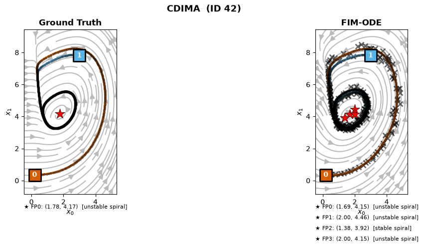
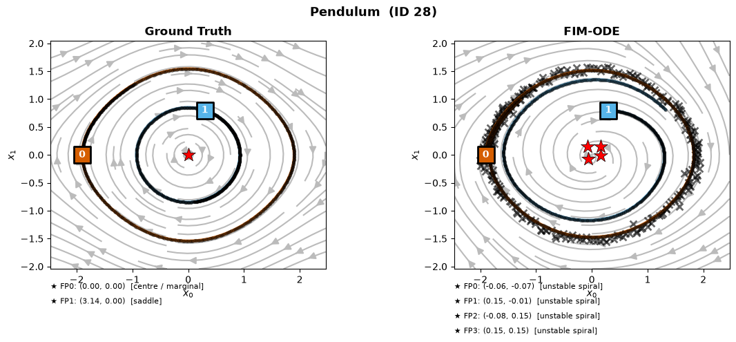
Visualise phase portraits with streamlines, integrated trajectories, and fixed point annotations.
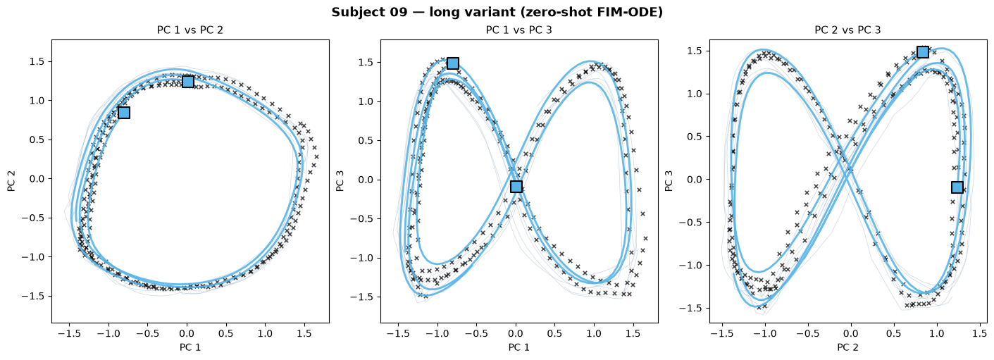
Apply FIM-ODE to real motion-capture data (CMU MoCap, Subject 09) and report zero-shot MSE in 50D joint-angle space.
import warnings
warnings.filterwarnings("ignore")
from transformers.utils import logging
logging.disable_progress_bar()
import numpy as np
import torch
import matplotlib.pyplot as plt
import sympy as sp
from ode_tutorial_helper import (
load_odebench_system,
make_fim_vf_fn,
find_fixed_points,
numerical_jacobian,
stability_analysis,
integrate_from_context,
)
device = 'cuda' if torch.cuda.is_available() else 'cpu'
print(f'Using device: {device}')Using device: cpu
1. Loading FIM-ODE
The pre-trained weights are hosted on the Hugging Face Hub at FIM4Science/fim-ode. The first call downloads and caches the model; subsequent calls load from the local cache.
from fim.models.ode import load_fim_ode_hf

model = load_fim_ode_hf(device=device)
model.eval()
print(f'Parameters: {sum(p.numel() for p in model.parameters()):,}')
Parameters: 12,968,068
2. Loading ODEBench trajectories
ODEBench provides reference trajectories for each system integrated from multiple initial conditions. We download the benchmark JSON from the Hugging Face Hub and add 3 % multiplicative Gaussian noise with 50 % subsampling to simulate realistic observations. We use one noisy trajectory as context for FIM-ODE throughout.
from huggingface_hub import hf_hub_download

# Download the ODEBench system definitions (3.5 MB JSON, cached after first run)
odebench_json = hf_hub_download(
    repo_id='FIM4Science/odebench',
    filename='strogatz_extended.json',
    repo_type='dataset',
)
print(f'ODEBench JSON: {odebench_json}')
ODEBench JSON: /Users/patrickseifner/.cache/huggingface/hub/datasets--FIM4Science--odebench/snapshots/91909865498f5d4bd69ea575527fee50ad329ef4/strogatz_extended.json
SEED         = 0
SYSTEM_IDS   = [26, 42, 28]
SYSTEM_NAMES = {26: 'LV Competition', 42: 'CDIMA', 28: 'Pendulum'}
N_CONTEXT    = 1   # one noisy trajectory used as context throughout

systems = {}
for sid in SYSTEM_IDS:
    times, trajs, meta = load_odebench_system(
        sid,
        json_path=odebench_json,
        noise_sigma=0.03,
        subsample_fraction=0.5,
        rng=np.random.default_rng(SEED),
    )
    systems[sid] = dict(times=times[:N_CONTEXT], trajs=trajs[:N_CONTEXT], meta=meta)
    print(f'System {sid:>3d} ({SYSTEM_NAMES[sid]:<20s}):  '
          f'context = {N_CONTEXT} trajectory × {trajs.shape[1]} steps × {trajs.shape[2]}D')

# Also load clean (noise-free, full-resolution) trajectories for plotting and IC integration
clean_systems = {}
for sid in SYSTEM_IDS:
    ct, cy, _ = load_odebench_system(
        sid, json_path=odebench_json, noise_sigma=0.0, subsample_fraction=1.0,
        rng=np.random.default_rng(SEED),
    )
    clean_systems[sid] = dict(times=ct, trajs=cy)
System 26 (LV Competition ): context = 1 trajectory × 256 steps × 2D
System 42 (CDIMA ): context = 1 trajectory × 256 steps × 2D
System 28 (Pendulum ): context = 1 trajectory × 256 steps × 2D
3. Vector field inference — a first example
Before analysing fixed points, we demonstrate what FIM-ODE actually produces: a continuous vector field inferred from a single noisy trajectory. We use the CDIMA chemical oscillator (system 42) as our example.
Protocol:
Context: noisy trajectory 1 (3 % multiplicative noise, 50 % subsampled).
Prediction: integrate the inferred vector field from two clean initial conditions.
Evaluation: compare against the noiseless ground-truth trajectories.
Each panel below shows one initial condition. Gray × markers are the noisy context observations; the black dashed curve is the clean ground truth; the colored solid curve is the FIM-ODE prediction integrated with RK45.
# CDIMA (system 42): integrate from two clean initial conditions
_sid   = 42
_ctx   = systems[_sid]['trajs']         # (1, T_ctx, 2) — noisy context
_ctx_ts= systems[_sid]['times'][0,:,0]  # (T_ctx,)
_clean = clean_systems[_sid]            # noise-free trajectories

TRAJ_COLORS = ['#D55E00', '#56B4E9']
_n_ic = min(2, _clean['trajs'].shape[0])

_preds_cdima = []
for _k in range(_n_ic):
    _y0   = _clean['trajs'][_k, 0]
    _tev  = _clean['times'][_k, :, 0]
    _pred = integrate_from_context(model, _ctx, _ctx_ts, _y0, _tev, device)
    _preds_cdima.append(_pred)

fig, axes = plt.subplots(1, _n_ic, figsize=(6 * _n_ic, 5), constrained_layout=True)
fig.suptitle('CDIMA — FIM-ODE conditioned on one noisy trajectory', fontsize=13)
if _n_ic == 1:
    axes = [axes]

for _k, ax in enumerate(axes):
    _gt   = _clean['trajs'][_k]      # (T_clean, 2) — clean GT
    _pred = _preds_cdima[_k]         # (T_clean, 2) — FIM-ODE
    _noisy = _ctx[0]                 # (T_ctx, 2)   — noisy context points
    _c = TRAJ_COLORS[_k]

    ax.scatter(_noisy[:, 0], _noisy[:, 1],
               s=30, c='gray', marker='x', linewidths=1.5, alpha=0.6,
               zorder=2, label='noisy context (traj 1)')
    ax.plot(_gt[:, 0], _gt[:, 1], 'k--', lw=2, alpha=0.8,
            zorder=3, label=f'ground truth (IC {_k+1})')
    ax.plot(_pred[:, 0], _pred[:, 1], color=_c, lw=2.5, alpha=0.95,
            zorder=4, solid_capstyle='round', label=f'FIM-ODE (IC {_k+1})')
    ax.scatter(_pred[0, 0], _pred[0, 1], s=200, marker='s',
               facecolor=_c, edgecolors='black', linewidths=2, zorder=5)
    ax.text(_pred[0, 0], _pred[0, 1], str(_k), fontsize=10,
            ha='center', va='center', color='white', fontweight='bold', zorder=6)

    ax.set_title(f'Initial condition {_k + 1}', fontsize=11)
    ax.set_xlabel('$x_0$', fontsize=10)
    ax.set_ylabel('$x_1$', fontsize=10)
    ax.legend(fontsize=8, loc='best')
    ax.set_aspect('equal', adjustable='datalim')

plt.show()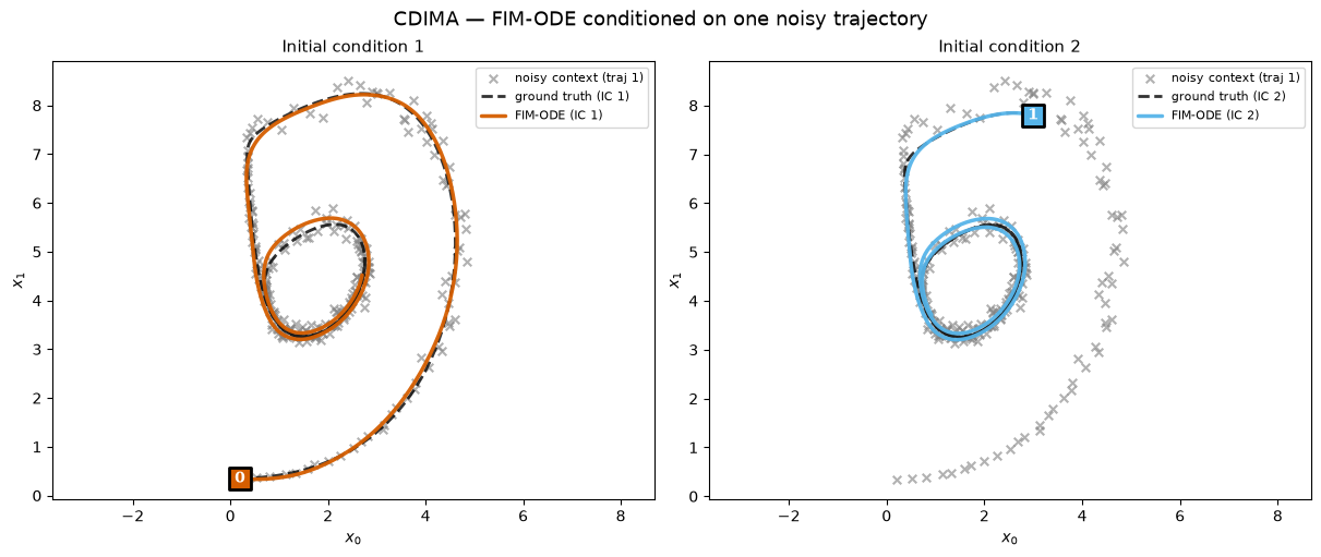
4. Ground-truth fixed points
A fixed point satisfies . Its stability is determined by the eigenvalues of the Jacobian :
| Eigenvalue pattern | Classification |
|---|---|
| All | stable node / spiral |
| All | unstable node / spiral |
| Mixed signs | saddle |
| Pure imaginary | centre / marginal |
We use SymPy to solve for fixed points and evaluate the Jacobian symbolically.
def sympy_fixed_points(eq_str, const_subs, label=''):
    """Symbolically find and classify fixed points of a 2-D ODE.

    Parameters
    ----------
    eq_str     : pipe-separated equation string, e.g. ``'x_1 | -c_0*sin(x_0)'``
    const_subs : list of constant values [c_0, c_1, ...]
    label      : printed header
    """
    eq_str = eq_str.replace('^', '**')
    parts  = [p.strip() for p in eq_str.split('|')]
    D      = len(parts)
    xs     = [sp.Symbol(f'x_{i}') for i in range(D)]
    cs     = {sp.Symbol(f'c_{i}'): v for i, v in enumerate(const_subs)}

    exprs  = [sp.sympify(p).subs(cs) for p in parts]
    J_sym  = sp.Matrix([[sp.diff(e, x) for x in xs] for e in exprs])

    try:
        fps_sym = sp.solve(exprs, xs, dict=True)
    except Exception:
        fps_sym = []

    results = []
    print(f'\n── {label} ──')
    for fp_dict in fps_sym:
        fp_num = np.array([complex(fp_dict.get(x, 0)) for x in xs])
        if np.any(np.abs(fp_num.imag) > 1e-8):
            continue
        fp_num = fp_num.real
        J_num  = np.array(J_sym.subs(fp_dict).evalf().tolist(), dtype=float)
        s      = stability_analysis(J_num)
        results.append(dict(fp=fp_num, J=J_num, **s))
        print(f'  x*  = {np.round(fp_num, 4)}   stability: {s["label"]}')
        print(f'  λ   = {np.round(s["eigenvalues"], 4)}')
    if not results:
        print('  No real fixed points found symbolically.')
    return results


gt_results = {}
for sid in SYSTEM_IDS:
    meta = systems[sid]['meta']
    gt_results[sid] = sympy_fixed_points(
        meta['eq'], meta['consts'],
        label=f'Ground truth — {SYSTEM_NAMES[sid]} (ID {sid})'
    )
── Ground truth — LV Competition (ID 26) ──
  x*  = [0. 0.]   stability: unstable node
  λ   = [3.+0.j 2.+0.j]
  x*  = [0. 2.]   stability: stable node
  λ   = [-2.+0.j -1.+0.j]
  x*  = [1. 1.]   stability: saddle
  λ   = [ 0.4142+0.j -2.4142+0.j]
  x*  = [3. 0.]   stability: stable node
  λ   = [-3.+0.j -1.+0.j]

── Ground truth — CDIMA (ID 42) ──
  x*  = [1.78   4.1684]   stability: unstable spiral
  λ   = [0.2415+1.712j 0.2415-1.712j]

── Ground truth — Pendulum (ID 28) ──
  x*  = [0. 0.]   stability: centre / marginal
  λ   = [0.+0.9487j 0.-0.9487j]
  x*  = [3.1416 0.    ]   stability: saddle
  λ   = [ 0.9487+0.j -0.9487+0.j]
5. FIM-ODE: encoding observations and finding fixed points
FIM-ODE encodes the noisy context trajectories once (a single forward pass through the transformer) and returns a neural vector field . We then search for its fixed points using a multi-start L-BFGS-B minimisation of .
fim_results = {}
for sid in SYSTEM_IDS:
    s   = systems[sid]
    vf  = make_fim_vf_fn(model, s['trajs'], s['times'], device=device)
    fps = find_fixed_points(vf, D=2, n_starts=400, x_range=(-6, 6),
                             rng=np.random.default_rng(SEED), top_k=4)
    fim_results[sid] = dict(vf=vf, fps=fps)

    print(f'\n── FIM-ODE — {SYSTEM_NAMES[sid]} (ID {sid}) ──')
    if not fps:
        print('  No fixed points found.')
    for fp, res in fps:
        J   = numerical_jacobian(vf, fp)
        s_i = stability_analysis(J)
        print(f'  x*  = {np.round(fp, 4)}   ||f(x*)|| = {res:.2e}   stability: {s_i["label"]}')
        print(f'  λ   = {np.round(s_i["eigenvalues"], 4)}')
── FIM-ODE — LV Competition (ID 26) ──
  x*  = [0.7692 1.0769]   ||f(x*)|| = 2.15e-01   stability: saddle
  λ   = [ 0.0303+0.j -2.0174+0.j]
  x*  = [0.4615 1.3846]   ||f(x*)|| = 2.15e-01   stability: saddle
  λ   = [ 0.1075+0.j -1.5373+0.j]
  x*  = [-0.1538  2.    ]   ||f(x*)|| = 2.18e-01   stability: stable node
  λ   = [-1.4659+0.j -2.2542+0.j]
  x*  = [1.0769 0.4615]   ||f(x*)|| = 2.39e-01   stability: stable node
  λ   = [-1.3092+0.j -0.0502+0.j]

── FIM-ODE — CDIMA (ID 42) ──
  x*  = [1.6923 4.1538]   ||f(x*)|| = 3.70e-01   stability: unstable spiral
  λ   = [0.5919+2.1629j 0.5919-2.1629j]
  x*  = [2.     4.4615]   ||f(x*)|| = 5.25e-01   stability: unstable spiral
  λ   = [0.5834+1.6939j 0.5834-1.6939j]
  x*  = [1.3846 3.9248]   ||f(x*)|| = 6.53e-01   stability: stable spiral
  λ   = [-0.5065+2.2871j -0.5065-2.2871j]
  x*  = [2.     4.1538]   ||f(x*)|| = 6.76e-01   stability: unstable spiral
  λ   = [0.4716+1.7578j 0.4716-1.7578j]

── FIM-ODE — Pendulum (ID 28) ──
  x*  = [-0.0613 -0.0686]   ||f(x*)|| = 9.05e-03   stability: unstable spiral
  λ   = [0.0361+0.1534j 0.0361-0.1534j]
  x*  = [ 0.1538 -0.0091]   ||f(x*)|| = 3.59e-02   stability: unstable spiral
  λ   = [0.1119+0.3206j 0.1119-0.3206j]
  x*  = [-0.0769  0.1538]   ||f(x*)|| = 9.86e-02   stability: unstable spiral
  λ   = [0.1644+0.6794j 0.1644-0.6794j]
  x*  = [0.1538 0.1538]   ||f(x*)|| = 1.08e-01   stability: unstable spiral
  λ   = [0.1205+0.4795j 0.1205-0.4795j]
6. Stability comparison
The table below compares the fixed points found by FIM-ODE against the ground truth.
header = f"{'System':<22} {'Model':<12} {'Fixed point':<22} {'Stability':<22} {'max Re(λ)':>10} {'||f(x*)||':>12}"
print(header)
print('-' * len(header))

for sid in SYSTEM_IDS:
    name = f'{SYSTEM_NAMES[sid]} ({sid})'

    gt_rows = [
        dict(fp=r['fp'], label=r['label'], max_real=r['max_real'], res=float('nan'))
        for r in gt_results[sid]
    ]
    fim_rows = [
        dict(fp=fp,
             label=stability_analysis(numerical_jacobian(fim_results[sid]['vf'], fp))['label'],
             max_real=stability_analysis(numerical_jacobian(fim_results[sid]['vf'], fp))['max_real'],
             res=res)
        for fp, res in fim_results[sid]['fps']
    ]

    for model_name, rows in [('GT', gt_rows), ('FIM-ODE', fim_rows)]:
        for i, r in enumerate(rows):
            tag   = name       if i == 0 else ''
            mname = model_name if i == 0 else ''
            fp_s  = '[' + ', '.join(f'{v:.3f}' for v in r['fp']) + ']'
            res_s = f"{r['res']:.2e}" if not np.isnan(r['res']) else '  (exact)'
            print(f"{tag:<22} {mname:<12} {fp_s:<22} {r['label']:<22} {r['max_real']:>+10.4f} {res_s:>12}")
    print()
System Model Fixed point Stability max Re(λ) ||f(x*)||
---------------------------------------------------------------------------------------------------------
LV Competition (26) GT [0.000, 0.000] unstable node +3.0000 (exact)
[0.000, 2.000] stable node -1.0000 (exact)
[1.000, 1.000] saddle +0.4142 (exact)
[3.000, 0.000] stable node -1.0000 (exact)
LV Competition (26) FIM-ODE [0.769, 1.077] saddle +0.0303 2.15e-01
[0.462, 1.385] saddle +0.1075 2.15e-01
[-0.154, 2.000] stable node -1.4659 2.18e-01
[1.077, 0.462] stable node -0.0502 2.39e-01
CDIMA (42) GT [1.780, 4.168] unstable spiral +0.2415 (exact)
CDIMA (42) FIM-ODE [1.692, 4.154] unstable spiral +0.5919 3.70e-01
[2.000, 4.462] unstable spiral +0.5834 5.25e-01
[1.385, 3.925] stable spiral -0.5065 6.53e-01
[2.000, 4.154] unstable spiral +0.4716 6.76e-01
Pendulum (28) GT [0.000, 0.000] centre / marginal +0.0000 (exact)
[3.142, 0.000] saddle +0.9487 (exact)
Pendulum (28) FIM-ODE [-0.061, -0.069] unstable spiral +0.0361 9.05e-03
[0.154, -0.009] unstable spiral +0.1119 3.59e-02
[-0.077, 0.154] unstable spiral +0.1644 9.86e-02
[0.154, 0.154] unstable spiral +0.1205 1.08e-01
7. Phase portraits
For each system we show a 1 × 2 figure (Ground Truth | FIM-ODE).
Style matches the paper figures:
Gray streamlines — the inferred (or true) vector field.
Green trajectory — integrated from initial condition 1.
Tomato trajectory — integrated from initial condition 2.
Black × (FIM-ODE panel only) — the noisy context observations.
Red ★ — fixed points found by the respective model.
Fixed point coordinates and stability labels are annotated below each panel.
COLORS  = ['#D55E00', '#56B4E9']
N_GRID  = 25


def _streamplot(ax, vf, xlim, ylim):
    x0g = np.linspace(*xlim, N_GRID)
    x1g = np.linspace(*ylim, N_GRID)
    X0, X1 = np.meshgrid(x0g, x1g)
    pts = np.stack([X0.ravel(), X1.ravel()], axis=-1)
    try:
        dX = vf(pts)
        U  = dX[:, 0].reshape(N_GRID, N_GRID)
        V  = dX[:, 1].reshape(N_GRID, N_GRID)
        ax.streamplot(x0g, x1g, U, V, color='#bbbbbb', density=0.9,
                      linewidth=1.5, arrowsize=1.5)
    except Exception as e:
        ax.text(0.5, 0.5, f'VF error:\n{e}', transform=ax.transAxes,
                ha='center', va='center', fontsize=8)


def _draw_panel(ax, trajs, fps=None, noisy_ctx=None):
    if noisy_ctx is not None:
        ax.scatter(noisy_ctx[:, 0], noisy_ctx[:, 1],
                   s=50, c='black', marker='x', linewidths=2, alpha=0.6, zorder=3)
    for k, traj in enumerate(trajs):
        if traj is None or np.any(np.isnan(traj)):
            continue
        c = COLORS[k]
        ax.plot(traj[:, 0], traj[:, 1], color=c, lw=3, alpha=0.9,
                zorder=4, solid_capstyle='round')
        ax.scatter(traj[:, 0], traj[:, 1], s=8, color='black', alpha=0.35, zorder=5)
        ax.scatter(traj[0, 0], traj[0, 1], s=280, marker='s',
                   facecolor=c, edgecolors='black', linewidths=2, zorder=6)
        ax.text(traj[0, 0], traj[0, 1], str(k), fontsize=10,
                ha='center', va='center', color='white', fontweight='bold', zorder=7)
    if fps:
        for fp, _ in fps:
            ax.scatter(fp[0], fp[1], s=220, c='red', marker='*',
                       edgecolors='k', linewidths=0.5, zorder=8)


def _fp_annotation(ax, fps, fontsize=8):
    """Write fixed-point coordinates and stability below the panel."""
    if not fps:
        ax.text(0.0, -0.06, 'no fixed points found',
                transform=ax.transAxes, ha='left', va='top',
                fontsize=fontsize, style='italic', color='gray', clip_on=False)
        return
    for i, (fp, label) in enumerate(fps):
        coord = '(' + ', '.join(f'{v:.2f}' for v in fp) + ')'
        ax.text(0.0, -0.06 - i * 0.065, f'\u2605 FP{i}: {coord}  [{label}]',
                transform=ax.transAxes, ha='left', va='top',
                fontsize=fontsize, color='black', clip_on=False)


# Build GT vector-field callables from the ODEBench equations
def _make_gt_vf(eq_str, consts, D=2):
    eq_str = eq_str.replace('^', '**')
    xs = [sp.Symbol(f'x_{i}') for i in range(D)]
    cs = {sp.Symbol(f'c_{i}'): float(v) for i, v in enumerate(consts)}
    parts = [sp.sympify(p.strip()).subs(cs) for p in eq_str.split('|')]
    funcs = [sp.lambdify(xs, expr, modules='numpy') for expr in parts]
    def vf(x):
        cols = [x[:, i] for i in range(D)]
        outs = []
        for func in funcs:
            v = func(*cols)
            if np.isscalar(v): v = np.full(x.shape[0], float(v))
            outs.append(np.asarray(v, dtype=float))
        return np.stack(outs, axis=-1)
    return vf

gt_vfs = {sid: _make_gt_vf(systems[sid]['meta']['eq'], systems[sid]['meta']['consts'])
          for sid in SYSTEM_IDS}

# Pre-compute FIM-ODE trajectories from clean ICs for every system
fim_phase_preds = {}
for sid in SYSTEM_IDS:
    ctx_traj = systems[sid]['trajs']            # (1, T_ctx, 2)
    ctx_ts   = systems[sid]['times'][0, :, 0]   # (T_ctx,)
    cs       = clean_systems[sid]
    preds    = []
    for k in range(min(2, cs['trajs'].shape[0])):
        y0  = cs['trajs'][k, 0]
        tev = cs['times'][k, :, 0]
        try:
            preds.append(integrate_from_context(model, ctx_traj, ctx_ts, y0, tev, device))
        except RuntimeError as e:
            print(f'  system {sid} IC{k}: {e}')
            preds.append(None)
    fim_phase_preds[sid] = preds

# One figure per system
for sid in SYSTEM_IDS:
    name  = SYSTEM_NAMES[sid]
    cs    = clean_systems[sid]
    noisy = systems[sid]['trajs'][0]   # (T_ctx, 2) — the noisy context traj

    gt_trajs  = [cs['trajs'][k] for k in range(min(2, cs['trajs'].shape[0]))]
    fim_trajs = fim_phase_preds[sid]

    # Shared axis limits derived from all trajectories
    all_t = [t for t in gt_trajs + fim_trajs if t is not None]
    all_x0 = np.concatenate([t[:, 0] for t in all_t])
    all_x1 = np.concatenate([t[:, 1] for t in all_t])
    pad0 = max((all_x0.max() - all_x0.min()) * 0.15, 0.5)
    pad1 = max((all_x1.max() - all_x1.min()) * 0.15, 0.5)
    xlim = (float(all_x0.min() - pad0), float(all_x0.max() + pad0))
    ylim = (float(all_x1.min() - pad1), float(all_x1.max() + pad1))

    gt_fps  = [(tuple(r['fp']), r['label']) for r in gt_results[sid]]
    fim_fps = [(tuple(fp),
                stability_analysis(numerical_jacobian(fim_results[sid]['vf'], fp))['label'])
               for fp, _ in fim_results[sid]['fps']]

    fig, axes = plt.subplots(1, 2, figsize=(12, 5))
    plt.subplots_adjust(left=0.07, right=0.97, top=0.88, bottom=0.22, wspace=0.18)
    fig.suptitle(f'{name}  (ID {sid})', fontsize=13, fontweight='bold')

    for ax, vf, panel_title in zip(axes,
                                    [gt_vfs[sid], fim_results[sid]['vf']],
                                    ['Ground Truth', 'FIM-ODE']):
        _streamplot(ax, vf, xlim, ylim)
        ax.set_xlim(xlim)
        ax.set_ylim(ylim)
        ax.set_aspect('equal', adjustable='box')
        ax.set_xlabel('$x_0$', fontsize=10)
        ax.set_ylabel('$x_1$', fontsize=10)
        ax.set_title(panel_title, fontsize=12, fontweight='bold')

    _draw_panel(axes[0], gt_trajs,  fps=gt_fps)
    _draw_panel(axes[1], fim_trajs, fps=fim_fps, noisy_ctx=noisy)

    fig.canvas.draw()
    _fp_annotation(axes[0], gt_fps)
    _fp_annotation(axes[1], fim_fps)

    plt.show()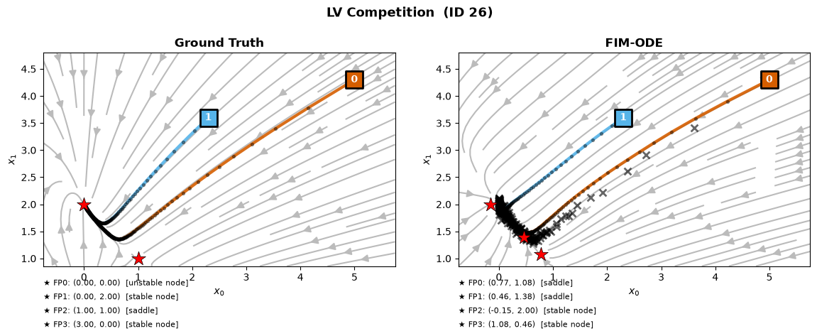
8. Motion Capture: CMU MoCap Subject 09
We now apply FIM-ODE to real motion-capture data from the CMU MoCap database, following the evaluation protocol of Hegde et al. (UAGP-ODE).
Data pipeline:
Raw 50D joint-angle time series are dimensionality-reduced to 5D via PCA fitted on the training set, then normalized per component to unit std.
FIM-ODE is limited to \leq 3$, so we feed it the first 3 PCA components.
Predictions are integrated from the test initial conditions and back-projected to 50D joint-angle space for evaluation.
We show two context lengths for Subject 09:
| Variant | Training trajectories | Train length | Test trajectories | Test length |
|---|---|---|---|---|
| short | 6 × 50 steps | 0.5 s | 2 × 120 steps | 1.2 s |
| long | 6 × 100 steps | 1.0 s | 2 × 120 steps | 1.2 s |
from ode_tutorial_helper import mocap_pca_to_50d, plot_mocap_pca

# Download preprocessed subject-09 data from HuggingFace (cached after first run)
mocap_short_path = hf_hub_download(
    repo_id='FIM4Science/fim-ode-mocap-tutorial',
    filename='mocap09_short.npz',
    repo_type='dataset',
)
mocap_long_path = hf_hub_download(
    repo_id='FIM4Science/fim-ode-mocap-tutorial',
    filename='mocap09_long.npz',
    repo_type='dataset',
)

def load_mocap_npz(path):
    d = np.load(path)
    return {
        'trn_ys':         d['trn_ys'],          # (n_trn, T_trn, 5) normalized PCA
        'trn_ts':         d['trn_ts'],          # (T_trn,)
        'tst_ys':         d['tst_ys'],          # (n_tst, T_tst, 5) normalized PCA
        'tst_ts':         d['tst_ts'],          # (T_tst,)
        'pca_components': d['pca_components'],  # (5, 50)
        'pca_data_mean':  d['pca_data_mean'],   # (50,)
        'norm_mean':      d['norm_mean'],        # (1,1,5)
        'norm_std':       d['norm_std'],         # (1,1,5)
    }

mocap = {
    'short': load_mocap_npz(mocap_short_path),
    'long':  load_mocap_npz(mocap_long_path),
}

for v, d in mocap.items():
    print(f'{v:6s}  trn: {d["trn_ys"].shape}  tst: {d["tst_ys"].shape}')
short   trn: (6, 50, 5)  tst: (2, 120, 5)
long    trn: (6, 100, 5)  tst: (2, 120, 5)
8.1 Integrating test trajectories
We condition FIM-ODE on all training trajectories (first 3 PCA components), then integrate from each test initial condition using RK45.
N_PCA     = 3   # FIM-ODE is limited to D ≤ 3
N_TEST    = 2   # number of test trajectories to show
preds_mocap = {}

for variant, d in mocap.items():
    ctx_traj = d['trn_ys'][:, :, :N_PCA]   # (n_trn, T_trn, 3)
    ctx_ts   = d['trn_ts']
    tst_ts   = d['tst_ts']

    preds = []
    for i in range(min(N_TEST, d['tst_ys'].shape[0])):
        y0   = d['tst_ys'][i, 0, :N_PCA].astype(float)
        pred = integrate_from_context(model, ctx_traj, ctx_ts, y0, tst_ts, device)
        preds.append(pred)   # (T_tst, 3)
    preds_mocap[variant] = preds
    print(f'{variant:6s}  integrated {len(preds)} test trajectories  '
          f'shape: {preds[0].shape}')
short integrated 2 test trajectories shape: (120, 3)
long integrated 2 test trajectories shape: (120, 3)
8.2 PCA projection plots
Each panel shows a 2D projection of the 3D PCA space.
Light blue lines: training context trajectories
Black ×: ground-truth test trajectories
Green lines + square: FIM-ODE prediction from the test IC
for variant, d in mocap.items():
    fig = plot_mocap_pca(
        trn_ys = d['trn_ys'][:, :, :N_PCA],
        tst_ys = d['tst_ys'][:, :, :N_PCA],
        preds  = preds_mocap[variant],
        title  = f'Subject 09 — {variant} variant (zero-shot FIM-ODE)',
        n_test = N_TEST,
    )
    plt.show()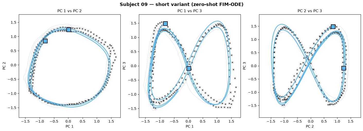
8.3 Zero-shot MSE (50D joint-angle space)
We back-project the 3D predictions to the full 50D joint-angle space (padding unmodelled PCA components 4–5 with zeros) and compute MSE against the ground-truth 50D trajectories.
print(f'  {"Variant":<10} {"n_trn":>6} {"T_trn":>6} {"n_tst":>6} {"T_tst":>6} {"MSE (50D)":>12}')
print('  ' + '-' * 48)

for variant, d in mocap.items():
    tst_ys_5d = d['tst_ys']   # (n_tst, T_tst, 5) — full 5D normalized PCA
    kw = dict(
        pca_components = d['pca_components'],
        pca_data_mean  = d['pca_data_mean'],
        norm_mean      = d['norm_mean'],
        norm_std       = d['norm_std'],
    )

    mses = []
    for i, pred_3d in enumerate(preds_mocap[variant]):
        pred_50d = mocap_pca_to_50d(pred_3d, n_dims=N_PCA, **kw)   # (T_tst, 50)
        true_50d = mocap_pca_to_50d(tst_ys_5d[i], n_dims=5, **kw)  # (T_tst, 50)
        mses.append(float(np.mean((pred_50d - true_50d) ** 2)))

    mse = float(np.mean(mses))
    n_trn, T_trn = d['trn_ys'].shape[:2]
    n_tst, T_tst = d['tst_ys'].shape[:2]
    print(f'  {variant:<10} {n_trn:>6d} {T_trn:>6d} {n_tst:>6d} {T_tst:>6d} {mse:>12.5f}')
Variant n_trn T_trn n_tst T_tst MSE (50D)
------------------------------------------------
short 6 50 2 120 6.10087
long 6 100 2 120 7.34162
Summary
With a single forward pass, FIM-ODE recovers vector fields that:
Match the ground-truth flow topology on ODEBench systems (correct qualitative structure)
Locate fixed points to within a fraction of a unit and classify their stability
Track real motion-capture trajectories in 3D PCA space with low MSE in the full 50D signal
This is achieved without any parameter fitting at test time, using only a few noisy or short-context trajectories as input.